APPS • DAILYTECH.ID - Manually toggling the display settings in Google Sheets is the simplest way to reveal the underlying computational logic of your spreadsheet cells.
To show all formulas in Google Sheets, navigate to the View menu, select Show, and then click Formulas. Alternatively, use the keyboard shortcut: Ctrl + ~ (Windows/ChromeOS) or ⌘ + ~ (Mac). This toggles the display between resulting values and the underlying formulas, aiding in debugging and reviewing complex spreadsheets efficiently. Understanding these methods is crucial for anyone who needs to audit or troubleshoot extensive data models.
The Core Method: How to Show Formulas in Google Sheets Using the Menu
For data analysts, educators, and users who rely on precise auditing, understanding the manual menu path to display formulas is foundational. While keyboard shortcuts are faster, the menu option is the guaranteed, universally recognized method for how to display formulas in Google Sheets, ensuring that even if a shortcut fails or is misremembered, you can still view the critical computational syntax. This process allows you to instantly transform a sheet full of results (like $45.00, 150, or TRUE) into a detailed logic map showing exactly what calculation is occurring in every cell (e.g., =B2*C2, =SUM(A:A), or =IF(D5>100,"TRUE","FALSE")).
Step-by-Step Guide to Toggle Formula Display
This systematic approach is essential when you need to show all formulas in Google Sheets simultaneously for a full-scale review or debugging session.
- Locating the View Menu: Begin by navigating to the main Google Sheets menu bar located at the top of your browser window. Look for the
Viewoption, typically positioned between theInsertandFormatmenus. ClickingViewopens a comprehensive dropdown menu dedicated to controlling how data and elements are presented on your screen. - Navigating to the Show Submenu: Within the
Viewmenu, hover your cursor over theShowoption. This action reveals a secondary menu containing various visibility controls, such as toggling gridlines, protected ranges, and, most importantly, the underlying formulas. - Selecting the Formulas Option: Click the
Formulasselection within theShowsubmenu. This single click acts as a global switch for the entire spreadsheet. Immediately, every cell that contains a calculation will reveal its exact formula instead of its computed result. Importantly, Google Sheets will automatically expand column widths to accommodate the full length of the formula text, preventing crucial syntax from being truncated or hidden.
To switch back to seeing the computed values, simply repeat the exact same three steps. The Formulas option acts as a toggle switch; if it is currently enabled (indicated by a checkmark next to it), clicking it will disable it and return the sheet to standard value view.
Accelerate Workflow: Show Formulas in Google Sheets Shortcut
When efficiency is paramount—as it often is for heavy spreadsheet users or those debugging massive sheets—relying on the menu path quickly becomes cumbersome. The dedicated Google Sheets show formulas shortcut is arguably one of the most powerful and time-saving shortcuts available, allowing instantaneous switching between the data view and the underlying logic view. Mastering this key combination drastically improves the speed at which you can audit, compare, and modify complex calculations.
This universal function is designed specifically to toggle the formula display. It is critical to note that this shortcut affects the entire spreadsheet view, not just selected cells.
Shortcuts for Windows and Mac
The specific keyboard shortcut relies on the tilde key (~), which is often associated with special characters but serves as the dedicated formula toggle in spreadsheet applications like Google Sheets and Microsoft Excel.
- Windows/ChromeOS Shortcut (
Ctrl + ~): Users on Windows or ChromeOS environments (including many laptops and desktops) should press and hold the Control key (Ctrl) and then press the tilde key (~). This immediate action activates the formula display. - Mac Shortcut (
⌘ + ~orControl +): Mac users have two options, depending on their keyboard layout and preference. The most common is pressing and holding the Command key (⌘) and the tilde key (~). On some extended Mac keyboards, especially if the tilde key is difficult to locate or access, the alternative combination ofControl +(Control plus the accent grave key) may also work, although⌘ + ~is the standardized Google Sheets shortcut for Mac users.
Note on the Tilde Key Location (~)
The tilde key (~) is usually located directly to the left of the 1 key, above the Tab key, on standard QWERTY keyboards. On certain international keyboard layouts, the tilde key might be a shifted key or located in a different position. If you are having trouble finding the key, look for the small squiggly line symbol. This symbol is often paired with the accent grave (“`) on the same keycap. Ensuring you hit this specific key is essential for the show formulas in google sheets shortcut to work correctly.
Viewing and Modifying a Single Formula
While toggling the formula view for the entire spreadsheet is vital for debugging the overall data flow, most day-to-day operations require inspecting or editing the calculation within just one or a few cells. When you need to view a formula in Google Sheets without disrupting the value view of the surrounding data, you rely on the Formula Bar or the cell editing mode.
The ability to quickly inspect a formula in a cell is foundational to confirming its logic, especially when troubleshooting an unexpected result.
How to View the Formula Bar in Google Sheets
The formula bar is a dedicated input and display area located above the column headers (A, B, C…) but below the menu bar. Its primary purpose is to show the exact content of the currently selected cell, whether that content is a static number, text, or a complex formula.
- Ensuring the Formula Bar is Visible: If you cannot see the formula bar, it may have been hidden unintentionally. To unhide formula bar in Google Sheets, navigate back to the
Viewmenu, selectShow, and ensure thatFormula barhas a checkmark next to it. If it is unchecked, click it once to reveal the bar. Keeping this area visible is critical for efficient single-cell editing. - Inspecting Cell Contents: When you click once on a cell that contains a formula, the formula bar immediately displays the underlying syntax. The cell itself continues to show the computed result, preserving the visual integrity of your output data while allowing you to inspect the logic.
- Editing vs. Viewing: You can modify the formula directly in the formula bar. When you finish editing, pressing Enter will update the formula and recalculate the result shown in the cell. Alternatively, you can double-click the cell itself to enter editing mode directly, allowing you to find formula in Google Sheets and edit it without having to look up to the formula bar.
Finding Specific Formulas
Sometimes, auditing involves checking every instance of a specific function—perhaps ensuring that every VLOOKUP is using the correct range, or every INDEX/MATCH combination is structured identically. If you need to search for formula text across your sheet without manually inspecting every cell, you can utilize the Find and Replace feature.
- Access the feature by navigating to the
Editmenu and selectingFind and Replace, or by using the shortcutCtrl + H(Windows) or⌘ + H(Mac). - In the
Findfield, enter the specific formula component you are looking for (e.g.,VLOOKUP,SUMIF, or even just a specific cell reference likeA10). - Crucially, ensure the “Search” range is set correctly (e.g., “All sheets” or “Specific range”).
- Expand the options area and check the box labeled “Search within formulas.” This forces Google Sheets to search the underlying syntax rather than the displayed values.
This method is invaluable for targeted audits, allowing you to instantly locate every cell where a particular function or argument is utilized.
Setting Up and Applying Formulas in Google Sheets
Before any user can effectively audit or show formulas in Google Sheets, they must first master the initial process of formula creation. Understanding the fundamental mechanics of how to do formulas in Google Sheets ensures that the resulting structure is logically sound and easily reviewable by others.
The application of formulas is the basis of any functional spreadsheet. Whether you are using a basic SUM function or complex array formulas, the entry requirements remain constant.
Initial Formula Input and Syntax Guide
Every computational entry in Google Sheets—whether simple arithmetic or a complex function—must adhere to a strict structure so the application knows to treat the input as logic, not static text.
- The Role of the Equals Sign (
=): The single most important rule is that all formulas must begin with the equals sign (=). This is the universal signal to Google Sheets that the content that follows is a calculation that must be evaluated and resolved, not simply displayed. If you forget the equals sign, the text of your intended formula will simply remain in the cell, and the calculation will never execute. - Utilizing Formula Guide and Auto-Suggestions: As you begin to type a function name (e.g.,
=SU), Google Sheets provides a powerful formula syntax guide via auto-suggestions. This addresses the need for clarity on how to show formula syntax in Google Sheets, offering real-time assistance. This guide helps you select the correct function and provides tooltip explanations of the required arguments (e.g.,range,criterion,sum_rangefor aSUMIF). Always reference this guide to ensure you are inputting arguments in the correct order, separated by commas.
How to Apply a Formula in Google Sheets
Once the formula is correctly entered in one cell (usually the top-left cell of the desired range), it is rarely necessary to manually add formula in Google Sheets to every subsequent cell.
- Selection and Entry: Type the complete formula into the first cell (e.g., cell C2).
- Using the Fill Handle: Click on cell C2. Notice the small square box (the fill handle) in the bottom-right corner of the cell outline.
- Dragging Down: Click and drag that fill handle downwards. Google Sheets automatically adjusts the relative cell references in your formula (e.g., B2 becomes B3, B4, B5, etc.), efficiently applying the calculation logic to hundreds of rows instantly. This auto-adjustment is often the source of errors, making the formula viewing toggle essential for confirming that the references are shifting correctly.
Device-Specific Viewing: How to Show Formulas on Mobile
As spreadsheet work increasingly shifts to flexible platforms, knowing how to interact with formulas on mobile devices becomes crucial. While the desktop environment offers convenient keyboard shortcuts for the formula toggle, the Google Sheets mobile app (on iPad, iPhone, or Android) presents formulas differently due to interface limitations.
There is no dedicated keyboard shortcut (like Ctrl + ~) available within the mobile app interface to show all formulas simultaneously. Therefore, the approach for how to show formulas in Google Sheets iPad or Android relies on individual cell inspection.
Viewing Formulas on Google Sheets Mobile App
The mobile interface is designed for data entry and immediate value review, prioritizing screen space over complex auditing tools.
- Tapping the Cell: To view the underlying formula, simply tap the cell containing the calculation.
- Display in the Edit Bar: When a cell is selected, the bottom of the screen typically shows the contents of that cell in a dedicated input field (the mobile equivalent of the desktop formula bar). If the cell contains a result (e.g., 500), the edit bar will reveal the actual formula (e.g.,
=A1+B1). - Editing Mode: Tapping the formula displayed in the edit bar opens the full keyboard and allows you to modify the calculation directly. This process is how to unhide cells in Google Sheets mobile, allowing interaction with the contents, even if they are lengthy.
Limitations of the Mobile Interface
It is important to understand that the mobile viewing mechanism is transactional—it only shows one formula at a time. If you need to audit hundreds of cells or compare formulas across multiple columns, the desktop application remains the vastly superior tool for full-scale review, leveraging the global formula toggle. Mobile is best reserved for quick checks or minor corrections.
Advanced Visualization: How to Show Equation of a Trendline in Google Sheets
Not all “formulas” exist within the standard spreadsheet grid. When dealing with advanced data analysis, particularly regression and forecasting, the equation that defines a trendline in a chart is essentially a dynamically generated mathematical formula derived from your input data. Knowing how to display this equation is crucial for communicating statistical findings.
If you are using a scatter plot or a line chart to visualize a relationship, Google Sheets can automatically calculate and display the linear regression equation (Y = mX + B) or other complex polynomials directly on the chart.
Steps to Display the Line Equation on a Chart
This process is handled entirely within the Chart Editor pane, which is separate from the main spreadsheet interface.
- Creating a Scatter Chart or Line Chart: Ensure your data is appropriately formatted for regression analysis (usually two columns of numerical data, X and Y). Insert a chart by going to
Insert>Chart, typically choosing a Scatter chart for best results. - Accessing Customization Settings: Double-click on the chart or click the three-dot menu in the upper right corner of the chart and select
Edit chart. This opens the Chart Editor sidebar. Navigate to theCustomizetab. - Adding a Trendline: In the
Customizemenu, scroll down and open theSeriessection. Locate and check the box toTrendline. By default, this adds a linear trendline. - Selecting the Equation Display: Once the trendline is visible, look within the same
Trendlinesettings subsection. Change theTypeif necessary (e.g., to Polynomial or Exponential). Then, under theLabeldropdown menu, select “Use Equation.” This instantly overlays the specific mathematical formula (how to show equation of a trendline in Google Sheets) that defines the line’s fit to your data. - Displaying R-squared: For rigorous analysis, it is also recommended to check the box for “Show R².” The R-squared value indicates how well the equation fits the data points (a value closer to 1.0 indicates a better fit), providing essential context for the trendline equation. This combination is how to show linear regression equation in Google Sheets effectively for academic or professional presentation.
Troubleshooting and Related Actions
When working with complex, multi-layered spreadsheets, debugging often involves not just viewing the formulas, but also managing the display settings to see only what is necessary, and ensuring no calculated data is inadvertently hidden.
Displaying Values Instead of Formulas
The most common “issue” after viewing formulas is forgetting how to show value instead of formula in Google Sheets and getting stuck in the auditing view. Fortunately, reversing the formula display is exactly the same action as enabling it.
To toggle back to the resulting values:
- Menu Reversal: Go to
View>Show>Formulas. If the option was checked, clicking it again will uncheck it, restoring the computed values to the cells. - Shortcut Reversal: Use the keyboard shortcut again:
Ctrl + ~(Windows/ChromeOS) or⌘ + ~(Mac). The shortcut functions purely as a toggle, switching the display state with every press.
If your sheet displays the formula text even though the formula toggle is off, verify that the cell does not have a leading apostrophe ('). A leading apostrophe forces the cell to treat the content as static text, ignoring the leading equals sign (=).
Managing Hidden and Unhide Cells in Google Sheets
Often, formulas that perform intermediate steps or helper calculations are placed in rows or columns that are then hidden from the main view to keep the presentation clean. If a calculation is producing an error or an unexpected result, these hidden areas might contain the root cause. Knowing how to view hidden cells in Google Sheets is paramount for thorough debugging.
To Unhide Rows or Columns:
- Locate the Gap: Look for a break in the row numbers or column letters (e.g., A, B, D, E, skipping C). Hidden cells are indicated by a slightly thickened line where the row or column header should be.
- Using the Context Menu: Click and drag to select the column letters or row numbers immediately surrounding the hidden area (e.g., select both Column B and Column D if C is hidden). Right-click on the selected headers. A menu will appear with the option to “Unhide column” or “Unhide row.”
- Using the Double-Line Icon: Alternatively, hover your cursor over the thickened line separating the visible headers. A small double-arrow icon will appear. Clicking this icon is the quickest way to unhide the cells in Google Sheets, instantly revealing the hidden intermediate data and formulas. This ensures that no part of the calculation chain remains obscured during the auditing process.
Conclusion
The ability to quickly toggle between seeing computed values and the underlying formulas is a cornerstone skill for anyone using Google Sheets for data management or complex modeling. Whether you utilize the systematic, multi-step process via the View menu or the instantaneous power of the Ctrl + ~ keyboard shortcut, mastering formula visibility transforms the often-challenging task of auditing and debugging complex spreadsheet logic into a swift, manageable operation. Understanding these mechanisms ensures accuracy, transparency, and efficiency in every data project.
FAQs – Show Formulas In Google Sheets
The universal shortcut to display or hide all formulas across your spreadsheet is Ctrl + ~ for Windows and ChromeOS users, or ⌘ + ~ for Mac users. This key combination acts as a toggle switch.
To inspect the formula of a single cell, simply click on the cell once. The complete, underlying formula syntax will immediately appear in the Formula Bar, located above the column headers.
This is the default view in Google Sheets, which displays the calculated result for readability. To switch this view and display the underlying formula text, you must use the View menu toggle or the keyboard shortcut.
Yes, but not all at once. On the mobile app, you must tap an individual cell, and the formula content will be displayed in the editing bar at the bottom of the screen for inspection and modification.
Use the Find and Replace feature (Ctrl + H or ⌘ + H). Enter the function name (e.g., SUMIF) in the Find field, then ensure you select the “Search within formulas” option in the expanded settings.