Have You Let Strangers Into Your Digital Camp? Here Is How to Lock Them Out

APPS • DAILYTECH.ID - To lock a sheet in Google Sheets, navigate to the target sheet, click the ‘Data’ menu, and select ‘Protected sheets and ranges.’ Click ‘+ Add a sheet or range,’ select ‘Sheet,’ choose the sheet you want to lock, and click ‘Set permissions.’ You can then restrict editing access to specific users or prevent all but yourself from modifying the protected data.

To protect data integrity and prevent unauthorized modifications, Google Sheets provides robust locking mechanisms for entire sheets, specific cells, or ranges. Understanding the nuances of these protection settings is crucial for maintaining accurate collaborative spreadsheets.

The Core Method: How to Protect an Entire Sheet from Editing

Data integrity is paramount in collaborative environments. When working with master data, historical records, or reference tables, preventing unauthorized changes is essential. The primary method for securing data in Google Sheets involves utilizing the built-in “Protected sheets and ranges” feature, which allows administrators to lock an entire sheet, thereby restricting modification rights across the entire tab. This addresses the core need of how to lock entire sheet in Google Sheets.

Step-by-Step Guide for Protecting a Single Sheet (Desktop/Web)

This detailed guide walks through the process of how to protect sheet in Google Sheets, restricting editing permissions for all users except designated collaborators. This method is the definitive way to implement a hard lock on a specific tab.

1. Preparation and Selection: Open your Google Sheet file. Locate and select the sheet tab you wish to lock (often referred to as how to lock a sheet tab in Google Sheets). Ensure you are on the correct sheet, as the locking mechanism is specific to the active tab.
2. Access the Data Menu: Navigate to the Data menu in the top toolbar. This menu houses the advanced features related to data management and security.
3. Initiate Protection: Select the Protected sheets and ranges option from the dropdown menu. A dedicated sidebar panel, labeled “Protected sheets and ranges,” will appear on the right side of your screen. This panel is the central hub for managing all protection rules within the entire workbook.
4. Define the Scope: Click the + Add a sheet or range button located at the top of the sidebar. In the rule creation interface, ensure the Sheet option is selected (as opposed to “Range”).
5. Specify the Target: From the subsequent dropdown menu, choose the specific sheet name (e.g., “Budget Summary,” “Raw Data,” or “Sheet2”) you want to protect.
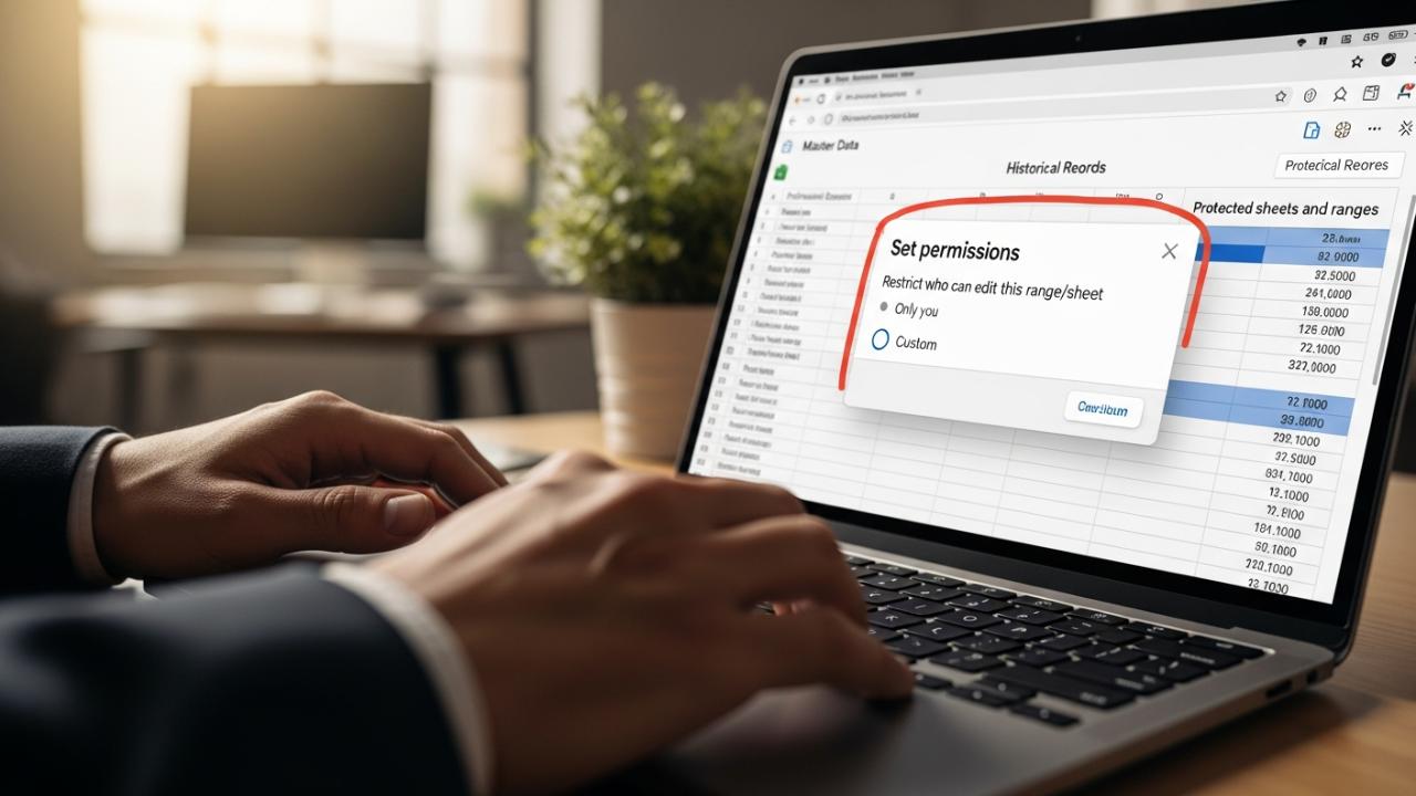
6. Configure Permissions: Once the sheet is selected, click the blue Set permissions button. This opens the crucial permissions dialogue box, which dictates who retains editing access.
7. Choose the Lock Type: Under the heading “Restrict who can edit this range/sheet,” you have two primary options for security:
   • Show a warning when editing this range (Soft Lock): This setting allows anyone with edit access to make changes, but they will receive a prominent pop-up warning message asking them to confirm their changes. This is useful for general collaboration rules but does not constitute a hard lock.
   • Restrict who can edit (Hard Lock): This is the option required for true protection.
     • If you select Only you, no other user—regardless of their overall sharing permissions for the file—will be able to modify the sheet. This is the simplest way to enforce a strict read-only status for collaborators.
     • If you select Custom, you can specify individual email addresses or Google Groups that will maintain editing rights, while everyone else will be locked out.
8. Finalize the Lock: Click Done to apply the protection rule. The rule will immediately take effect, and the protected sheet icon will appear in the sidebar list. Collaborators attempting to edit the protected sheet will receive an “Error” notification stating they do not have permission.

Locking Sheets on Mobile Devices (Android and iOS)

Business professionals and students often manage spreadsheets away from a desktop. Knowing how to lock sheet in Google Sheets mobile is vital for maintaining security while collaborating on the go. While the interface differs slightly from the desktop version, the underlying logic and permissions are identical.

1. Access the Mobile App: Open the Google Sheets app on your Android or iOS device and navigate to your specific file.
2. Locate the Target Sheet: Tap the sheet tab name (usually found at the bottom of the screen) you want to lock.
3. Open Protection Options: Tap the vertical three-dot menu icon adjacent to the sheet name (or sometimes found by long-pressing the tab name).
4. Select Protection: Select the Protect Sheet option from the context menu that appears.
5. Set Permissions: A new screen will load, allowing you to Set permissions. Here, you can configure the restrictions to “Only you” or “Custom,” mirroring the functionality of the desktop application.
6. Save Changes: Tap the checkmark or save icon to finalize the protection rule. This ensures that the protection is universally applied across all devices accessing the spreadsheet.

Locking Specific Areas: Cells, Ranges, Rows, and Columns

In many collaborative workflows, a sheet must remain open for data entry but secure in its structure. You may need to protect calculated results or vital headers. This highly specific control addresses how to lock a Google Sheet cell or google sheets how to lock cells from editing.

Protecting Individual Cells or Data Ranges

To maintain the integrity of key input points, you can lock specific ranges in Google Sheets from editing, enabling flexible collaboration while securing critical areas. This is often necessary when protecting lookup tables or reference data within a larger, editable sheet.

1. Select the Range: Using your cursor, highlight the specific cells or range (e.g., A1:C10) you wish to secure.
2. Initiate Range Protection: Go to Data > Protected sheets and ranges.
3. Define the Range Scope: Click + Add a sheet or range. Ensure the Range option is selected (it will automatically populate with the range you highlighted, but you can adjust it manually if needed).
4. Configure Restrictions: Click Set permissions.
5. Apply Security: Just as with sheet protection, you set the editing restrictions to “Only you,” “Custom,” or use the softer “Warning” option. For hard protection, selecting “Custom” and entering specific editor emails is the most common use case here.
6. Name the Rule (Optional but Recommended): In the sidebar, it is best practice to give the rule a clear description (e.g., “Protected Formulas 2026”) so you or other administrators know exactly what data is secured.

Locking Specific Rows or Columns

When managing data sets, the header row and certain identification columns (like timestamps or unique IDs) must never be altered. To ensure these foundational elements are preserved, the process for Google Sheets how to lock a column or Google Sheets how to lock a row is a straightforward extension of range protection.

1. Selection Method: Instead of highlighting a block of cells, click the gray header letter (e.g., Column A) or number (e.g., Row 1) to select the entire vertical or horizontal span.
2. Applying the Rule: Follow the standard steps for protecting individual ranges listed above (Data > Protected sheets and ranges).
3. Verification: The system will automatically register the entire column or row (e.g., A:A or 1:1) as the protected range. Apply the desired permissions and save the rule. This guarantees that no collaborator can accidentally delete or overwrite the foundational structure of your data table.

Ensuring Formula Integrity

A primary reason for locking specific cells is to secure calculations. Learning how to lock a cell in Google Sheets formula is vital to prevent collaborators from corrupting the core logic of the spreadsheet. If a user inputs data directly into a cell containing a complex array formula or a key VLOOKUP calculation, the entire structure can break.

• Identify Formula Cells: Carefully select all cells or ranges that contain essential formulas (e.g., total sums, dynamic outputs, or lookup functions).
• Implement Range Protection: Use the Protected sheets and ranges feature to apply “Only you” or “Custom” editing permissions specifically to the range containing the formulas.
• Strategic Protection: A common best practice is to lock the output cells (where the formulas reside) while leaving the input cells (where collaborators type raw data) completely unprotected. This balance ensures users can contribute while securing the underlying computational engine (Google Sheets how to lock formula).

Advanced Locking: Limiting Viewing and Password Protection

Google Sheets operates within the Google ecosystem, meaning its security model is fundamentally different from traditional desktop software like Microsoft Excel. This leads to frequent questions about dedicated security measures.

Can You Password Protect a Sheet in Google Sheets?

A common transactional search query is how to password lock a sheet in Google Sheets. It is crucial to understand the limitations: Currently, there is no direct feature to password lock a sheet in Google Sheets in the traditional sense, where a user must enter a password (like “1234”) to open or edit a locked tab.

The platform relies entirely on Google Account security, file sharing permissions, and the protection mechanisms detailed above. When users ask, can you password protect a sheet in Google Sheets, they are usually seeking a method to strictly control who can modify the sheet. The “Custom” permission setting serves as the functional equivalent of internal password protection, as it requires Google Account validation to bypass.

Restricting Viewing Access: A Note on File-Level Security

While the “Protected sheets and ranges” feature restricts editing, it does not restrict viewing. If a collaborator has ‘View’ access to the overall Google Sheet file, they will be able to see the data in a locked sheet.

To address how to lock a sheet in Google Sheets from viewing, you must manage the sharing settings at the Google Drive file level:

1. Go to the main sheet document.
2. Click the blue Share button in the top right corner.
3. Change a user’s permission from “Viewer” to “Restricted” or remove their access entirely. This controls viewing access for the entire workbook, as Google Sheets does not currently support hiding individual tabs based on user viewing permissions.

Restricting Editing Access to Specific Users Only

When setting permissions, the “Custom” option is the closest substitute for fine-grained, password-like security. This ensures that only specific, validated colleagues can modify the data, even if dozens of people have general edit access to the file.

1. In the Protected sheets and ranges sidebar, select the relevant rule (or create a new one).
2. Click Set permissions.
3. Select the “Restrict who can edit” radio button.
4. Choose Custom from the dropdown menu.
5. Input Authorized Editors: Carefully enter the exact Google email addresses of the specific users or groups who should retain editing rights.
6. Final Check: Ensure the list is accurate. All other users who have ‘Editor’ status for the main file but are not on this custom list will be barred from editing the protected sheet or range.

Managing and Unlocking Protected Sheets

Data requirements evolve quickly. You may need to grant temporary editing access for a mass update or permanently remove restrictions once a project phase is complete. Knowing how to unlock a locked sheet in Google Sheets is as important as knowing how to lock it.

How to Temporarily Modify Protection Settings

If a protected sheet needs a short window of collaborative editing, you do not need to delete the rule entirely.

1. Open the Protected sheets and ranges sidebar (Data > Protected sheets and ranges).
2. Click on the specific protection rule you wish to adjust.
3. Click Set permissions.
4. Temporarily change the restriction setting from “Only you” to “Custom” and add the required collaborator, or change it to “Show a warning.”
5. After the temporary collaboration period is over, restore the original, stricter protection setting.

How to Permanently Remove Protection from a Locked Sheet

If you need to permanently remove protect sheet in Google Sheets and revert the sheet to full collaborative access:

1. Open the Protected sheets and ranges sidebar by navigating to Data > Protected sheets and ranges.
2. Review the list of rules displayed in the sidebar. These rules list the protected ranges and sheets.
3. Locate the specific sheet or range protection rule you wish to delete.
4. Click the rule to open its details.
5. Look for the trash can icon (Delete protection rule) located in the upper right corner of the rule box.
6. Click the trash can icon and confirm the deletion. This action instantly removes the specific sheet protection and restores full editing access to all collaborators who have general edit permissions on the Google Sheet file. This is the only official method to how to unlock a locked sheet in Google Sheets.

FAQs – How to Lock a Sheet in Google Sheets